---

title: “Hilbert Curve Visualization with Manim” format: revealjs editor: visual —

Introduction

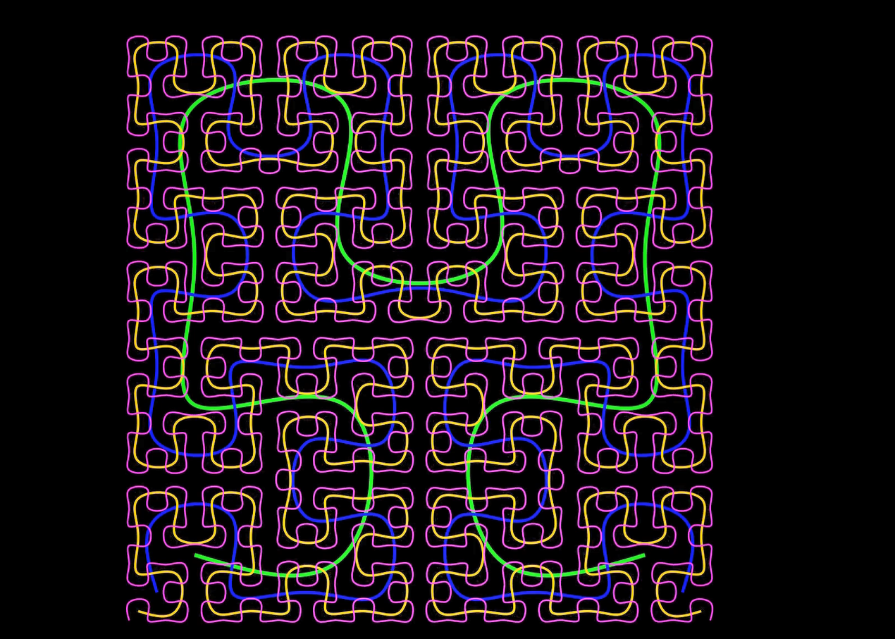
The Hilbert Curve algorithm generates a continuous fractal space-filling curve that passes through every point in a grid without crossing itself. It is used to preserve spatial locality, making it valuable in computer graphics, image processing, and data indexing.

Industry Applications: - Database Storage: Multidimensional data indexing - Memory Hierarchy Optimization: Improves cache efficiency and query performance - Geographic Information Systems (GIS): Maps multi-dimensional data to one dimension while maintaining proximity relationships

---

1. Setting Up the Scene

from manim import *

class HilbertCurve(Scene):
    def construct(self):
        self.camera.background_color = BLACK

• Scene: Base class for all animations.
• self.camera.background_color: Sets the background to black for better contrast.

Black Background for Better Contrast

---

2. Adding a Title

title = Text("Hilbert Curve Visualization", font_size=26, color=BLUE).to_edge(UP * 0.5)
self.play(Write(title))
self.wait(1)
self.play(FadeOut(title), run_time=2)

• Text(...): Creates a text object.
• to_edge(...): Moves it to the top.
• Write(...): Animates drawing the text.
• FadeOut(...): Fades the title before proceeding.

Title

---

3. Defining Styles

CURVE_COLORS = ["#FF0000", "#00FF00", "#0000FF", "#FFD700", "#FF00FF", "#00FFFF"]
STROKE_WIDTHS = [6, 5, 4, 3, 2, 1]

Each level of the curve gets its own color and decreasing stroke width for visual clarity.

---

4. Recursive Point Generation

def get_hilbert_points(level, offset=np.array([0, 0, 0]), size=4):
    ...

• Recursive function that constructs points for each level.
• Each quadrant applies transformation and translation based on its position.
• Combines all to build the full curve.

Initial Sketched Curve

---

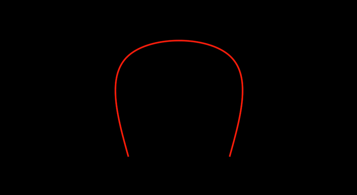
5. Constructing the Curves

max_level = 5
curves = []
for level in range(1, max_level + 1):
    points = get_hilbert_points(level)
    curve = VMobject(stroke_color=CURVE_COLORS[level-1], stroke_width=STROKE_WIDTHS[level-1])
    curve.set_points_smoothly(points)
    curves.append(curve)

• Generates a list of curves, each for a different level of the Hilbert curve.
• VMobject is used for vector graphics paths.

---

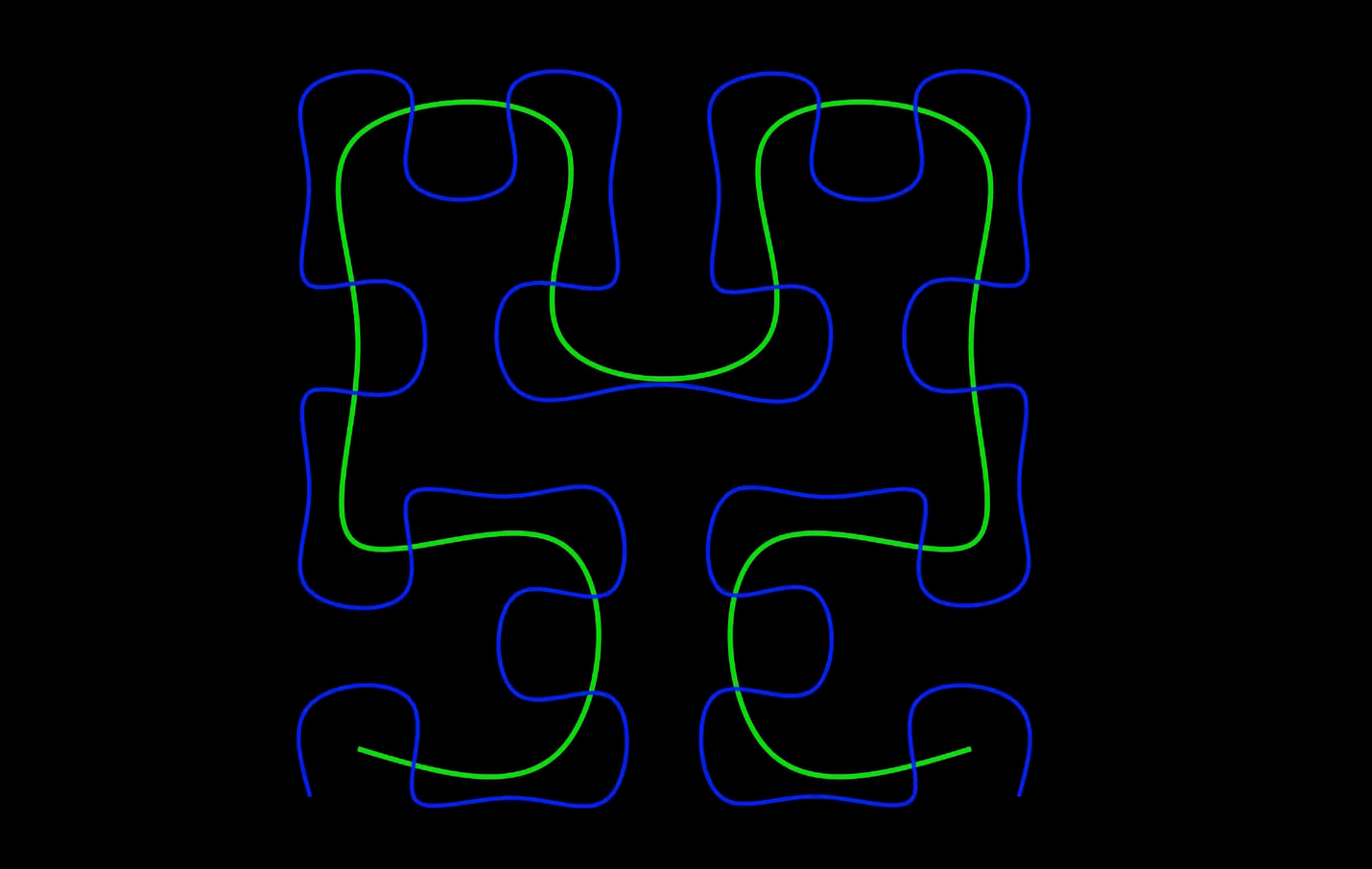
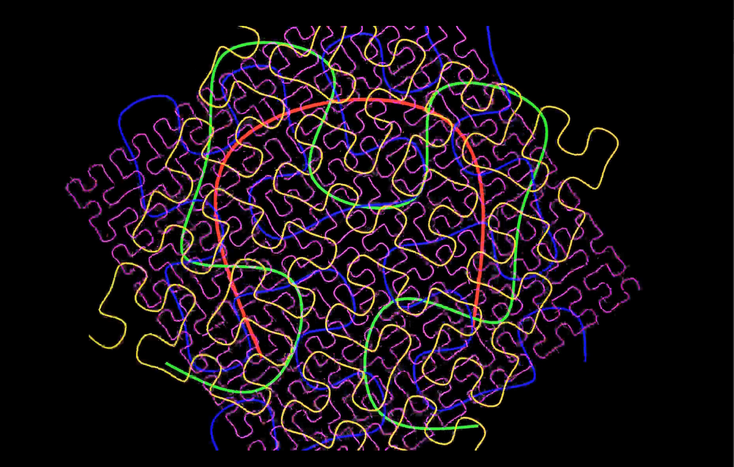
6. Animating the Transformation

self.play(Create(curves[0]), run_time=5)
for i in range(len(curves)-1):
    self.play(Transform(curves[i], curves[i+1]), run_time=4)

• Draws the level 1 curve.
• Uses Transform to morph each level into the next one.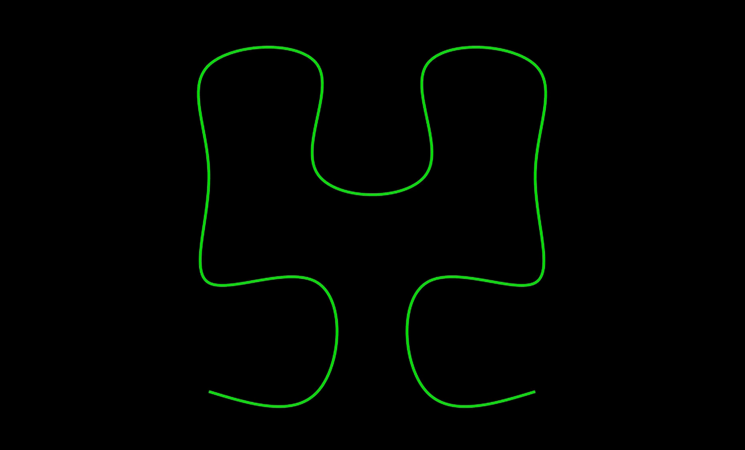

---

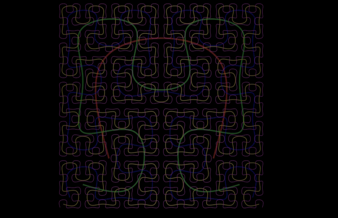
Level2 Sketched Curve

---

Level3 Sketched Curve

---

Level4 Sketched Curve

---

7. Scene Cleanup and Final Curves

self.clear()
for curve in curves:
    self.add(curve)

• Clears the scene to start a new phase.
• Adds the final versions of each level’s curve to the scene.

---

8. Rotation Animation

rotations_out = [Rotate(curve, angle=PI) for curve in curves]
rotations_back = [Rotate(curve, angle=-PI) for curve in curves]
self.play(*rotations_out)
self.play(*rotations_back)

• Rotates each curve forward and then back.
• *rotations_out means playing multiple animations in parallel.

Camera Rotations to Showcase Each Level of Animation

---

9. Dissolve / Fade Out

fade_animations = [FadeOut(curve, run_time=2) for curve in curves]
self.play(*fade_animations, rate_func=lambda t: smooth(t), run_time=3)

• Fades out all curves with a smooth effect to close the animation.

The Objects are Faded from the Scene

---

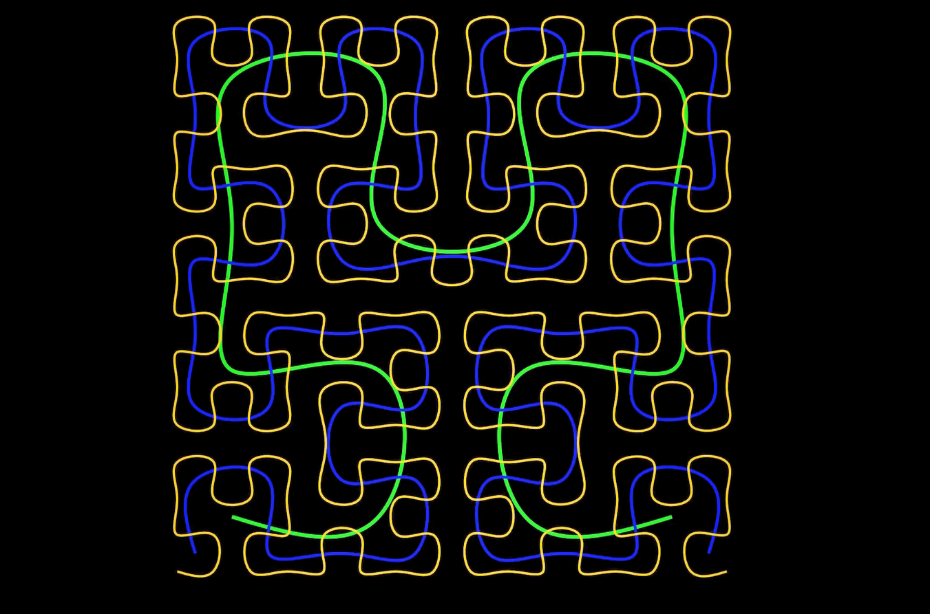
Summary

• Recursive generation enables fractal growth.
• Manim makes it easy to animate complex mathematical structures.
• The Hilbert Curve demonstrates how 1D lines can fill 2D space—a beautiful idea in computer graphics and data storage.